机器学习_3:无监督学习经典模型

可以算作是一种特征工程的办法了。他最重要的是发现数据本身的特点。功能如下：

• 发现数据的群落（聚类），寻找离群的样本
• 降维处理（PCA），保留低维且相关性高的特征

数据聚类

k均值算法

1. 导包+导数据集

import numpy as np
import matplotlib.pyplot as plt
import pandas as pd

digits_train = pd.read_csv('optdigits.tra', header=None)    # 不将文件中的第一行作为列名
digits_test = pd.read_csv('optdigits.tes', header=None)
print(digits_test.shape)
print(digits_train.shape)

观察形状不难看出，有65个特征，即64个为x，最后一个为y

2. 分割数据集

X_train = digits_train[np.arange(64)]
y_train = digits_train[64]

X_test = digits_test[np.arange(64)]
y_test = digits_test[64]

3. knn模型

from sklearn.cluster import KMeans

kmeans = KMeans(n_clusters=10)
kmeans.fit(X_train)

y_pred = kmeans.predict(X_test)

4. 模型评价

• ARI指标用于评估数据有所属类别

from sklearn import metrics

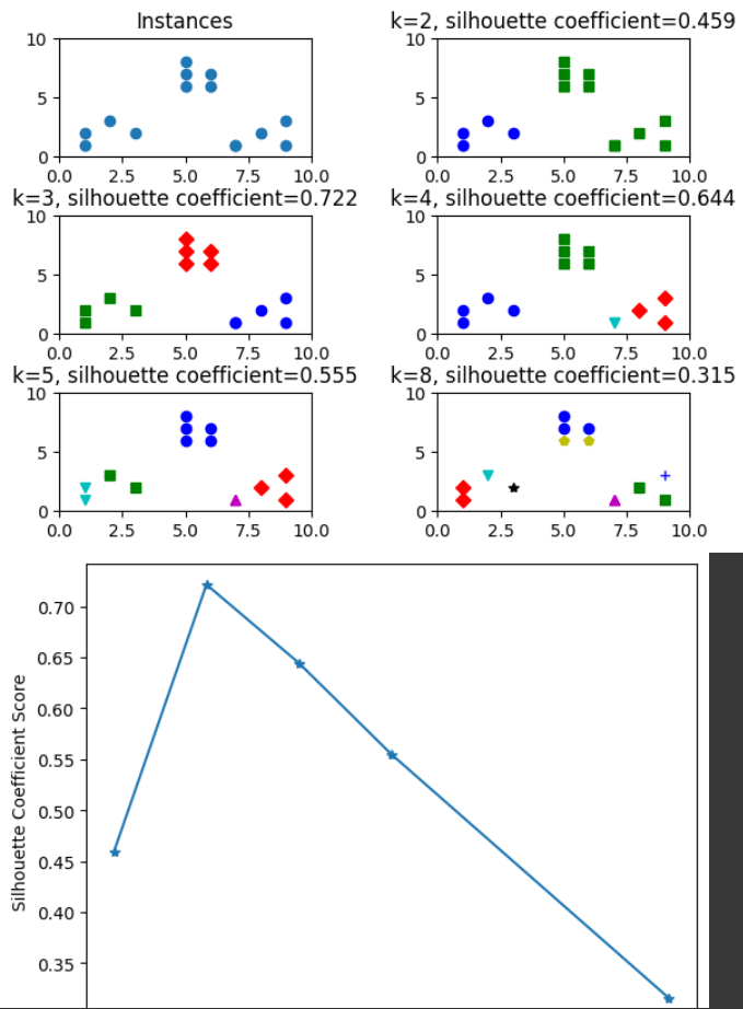
print("ARI:", metrics.adjusted_rand_score(y_test, y_pred))

• 没有所属类别时，使用轮廓系数，其取值为[-1, 1]越大说明聚类效果越好

from sklearn.metrics import silhouette_score

# 分割3*2=6个子图，并在1号子图作图
plt.subplot(3, 2, 1)

# 初始化原始数据点
x1 = np.array([1, 2, 3, 1, 5, 6, 5, 5, 6, 7, 8, 9, 7, 9])
x2 = np.array([1, 3, 2, 2, 8, 6, 7, 6, 7, 1, 2, 1, 1, 3])
X = np.array(list(zip(x1, x2))).reshape(len(x1), 2)

# 1号子图做出原始数据点阵的分布
plt.xlim([0, 10])
plt.ylim([0, 10])
plt.title('Instances')
plt.scatter(x1, x2)

colors = ['b', 'g', 'r', 'c', 'm', 'y', 'k', 'b']
markers = ['o', 's', 'D', 'v', '^', 'p', '*', '+']

clusters = [2, 3, 4, 5, 8]      # 簇的个数
subplot_counter = 1             # 子图编号
sc_scores = []                  # 存储每个簇对应的轮廓系数
# 循环聚类并绘制结果
for t in clusters:
  subplot_counter += 1
  plt.subplot(3, 2, subplot_counter)
  kmeans_model = KMeans(n_clusters=t).fit(X)

  for i, l in enumerate(kmeans_model.labels_):
    plt.plot(x1[i], x2[i], color=colors[l], marker=markers[l], ls='None')

  plt.xlim([0, 10])
  plt.ylim([0, 10])
  sc_score = silhouette_score(X, kmeans_model.labels_, metric='euclidean')
  sc_scores.append(sc_score)

  # 轮廓系数与不同类簇数量的直观显示图
  plt.title('k=%s, silhouette coefficient=%0.003f' %(t, sc_score))

# 调整子图之间的间距
plt.subplots_adjust(left=0.1, right=0.9, top=0.9, bottom=0.1, hspace=0.5, wspace=0.5)

# 轮廓系数与不同类簇数量的关系曲线
plt.figure()
plt.plot(clusters, sc_scores, '*-')
plt.xlabel('Numbers of Clusters')
plt.ylabel('Silhouette Coefficient Score')

plt.show()

效果如下：

knn也同时具有缺陷

• 容易收敛到局部最优解
• 需要预先设定簇的数量

此时介绍肘部法判断类簇个数，当曲线趋于平缓时，可认定最佳的k值(懒的敲代码了嘻嘻)

特征降维

主成分分析（PCA）

依然是手写字体的例子，通过PCA将64个维度压缩，依然可以发现绝大多数字之间的区别性